[03] Intensity Transformations and Spatial Filtering

Intensity transformation

이미지의 intensity를 변환하는 방법이다. $g(x,y) = T[f(x,y)]$

 

대표적으로 다음과 같은 방법이 있다.

• Linear : negative, identity
• Logarithmic : log, inverse-log
• Power law : $n^{th}$ power, $n^{th}$ root

 

Image Negatives

$$S = L - 1- r$$

Black dominant image에서 white 계열의 차이를 효과적으로 확인할 수 있다.

 

Log transformations

$$S = c \log (1+r)$$

Low intensity level을 wide하게 만드는 효과가 있다. 이 때문에, low intensity간의 차이는 강화되고 high intensity는 차이가 줄어들게 된다.

 

Power-law transformations

$$S=cr^{\gamma}$$

$$S=c(r+\epsilon)^{\gamma}$$

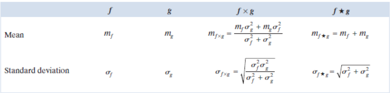
Image capture, printing, display에 맞춰 감마 보정으로 사용된다. 예를 들어 display의 감마가 x2.5이면 이미지의 감마를 1/2.5로 줄이면 완벽한 이미지가 나오게 된다.

또한 대비가 강조되는 효과도 있다.

 

Piecewise Linear transformations

Contrast Stretching

window level operation이다.

 

Intensity-level slicing

 

Bit-Plane slicing

특정 bit만 살리기, 별 차이가 없는 경우 Image compression에 유용함

 

Histogram Processing

Intensity $r_k$의 수를 $n_k$라고 하면, histogram은 다음처럼 표현할 수 있다.

$$h(r_k) = n_k$$

k=0,,,L-1

Normalization = $p(r_k) = {h(r_k) \over MN} = {n_k \over MN}$

 

$p(r_k)$는 해당 intensity의 확률이라고 볼 수 있다. (0~1) 보통 histogram을 말하면, normalized histogram을 의미하게 된다.

 

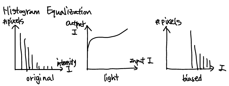
Histogram shape는 image appearance에 영향을 주기도 한다. 가령 wide range of intensity는 contrast 강조에 유용하다. 반대로 narrow histogram이면 contrast가 안좋음을 의미한다. 그럼 histogram을 잘 조정하면 더 좋은 이미지를 얻을 수 있음을 의미하게 된다.

 

Histogram Equalization(or linearization)

• r : [0, L-1]
• $s = T(r)$
• $T(r)$ 은 monotonic increasing function in $0 \leq r \leq L-1$
• $0 \leq T(r) \leq L-1$ for $0\leq r \leq L-1$

$T(r)$에 대한 이 조건이 맞지 않으면 intensity 역전(negative와 비슷)이 발생하거나 output의 range가 input과 같지 않는 일이 발생한다.

 

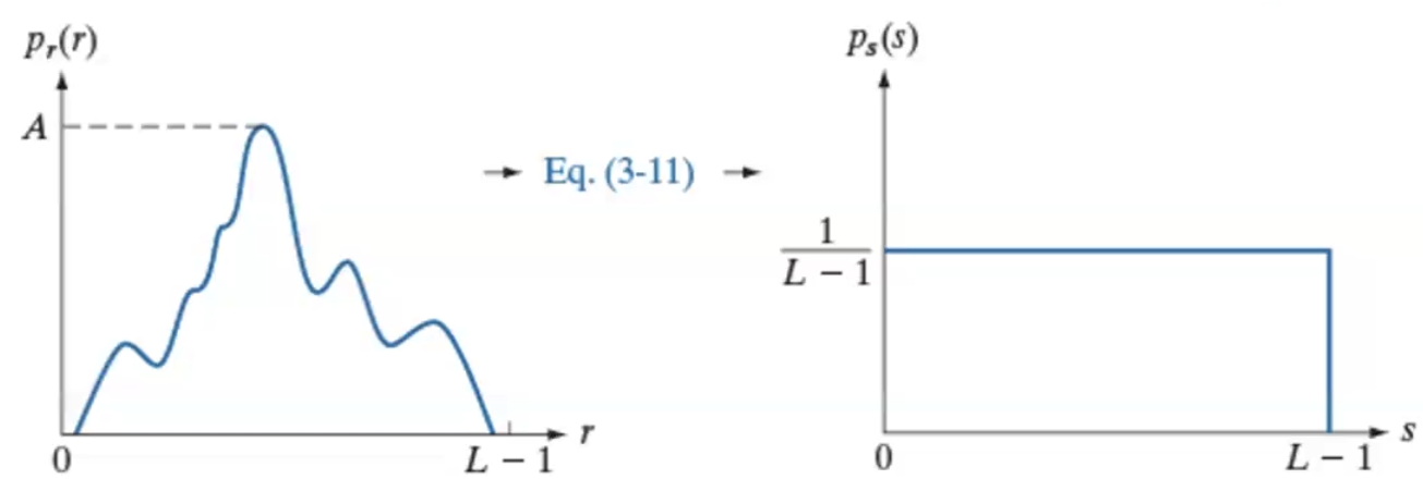
Intensity level을 random variable로 생각하면 $r$과 $s$에 대한 PDF를 다음처럼 표현할 수 있다.

$$P_s(s) = P_r(r)|{dr \over ds}|$$

 

그리고 만약 Transformation function, $T(r)$을 PDF의 CDF 정의하면,

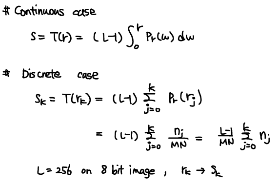
$$s = T(r) = (L-1) \int ^{r}_{0} P_r(w) dw$$

 

정리하면 $P_r(r)$에 상관없이 항상 $P_s(s) = P_r(r) {1 \over (L-1)P_r(r)} = {1 \over (L-1)}$이 된다. (uniform probability density function)

Histogram이 wide range를 가지게 변경된 것을 확인할 수 있다. = contrast가 좋아졌다.

 

실제로는 discrete한 값을 가지므로 다음처럼 표현한다.

Discrete한 경우는, 완벽하게 uniform distribution을 가지지는 않지만, 거의 비슷하다.

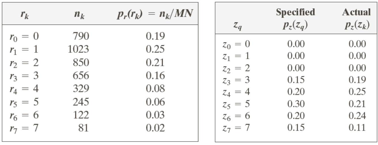
Example) 3-bit image, 64 by 64 pixels

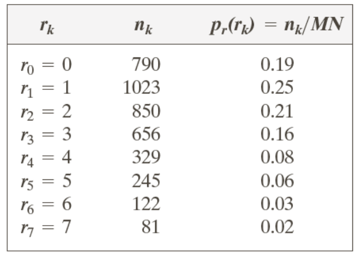
(1) $s_0 = (L-1) \sum _{j=0}^{0} p_r(r_0) = 7 * 0.19 = 1.33 => 1$

(2) ...

 

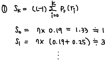
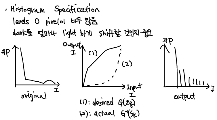
Histogram Matching(or specification)

Histogram equal.은 항상 좋은 결과를 주지 않는다. 가령, 특정 intensity가 매우 좁게 형성되길 바랄 경우 wide하게만 형성하는 histogram equal.은 좋지 않은 선택이다. 이를 해결하려는 것이 histogram matching이다.

 

Input $p_r(r)$이 $p_z(z)$로 나타나게 만드는 방법이다.

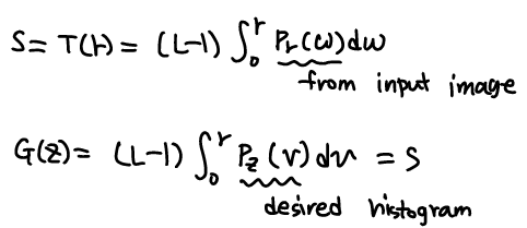
Histogram equal.에서 알 수 있듯이, PDF의 CDF를 transformation으로 사용하면 결과는 항상 같았고 $G(z)=s$를 이용해 histogram을 바꾸는 것이 목표이다.

 

How?
(1) $s=T(r)$ 구하기

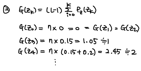
(2) $G(z)$ 구하기

(3) $G(z)=s$를 이용해서 $z=func(s)$ 구하기

(4) (1)의 결과를 이용해 $z=func(r)$ 구하기

(5) $z$와 $r$의 matching 가능

 

마찬가지로 discrete한 형태에 대해서는 approximation이 사용된다.

(1) $s_k = (L-1) \sum p_r(r_k)$ 구하기, $round(s_k)$

(2) $G(z_q) = (L-1) \sum p_z(z_q)$ 구하기, $round(G(z_q))$

(3) $z_q$ | $G(z_q)$ lookup table 생성

(4) $s_k$ -> $G(z_q)$ 값 맵핑

(5) $G(z_q)$의 $z_q$로 $s_k$를 가지는 $r_k$ 맵핑

 

$G(z_q)$의 값이 unique하지 않으면, 제일 작은 값으로 설정하게 된다.

 

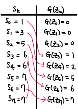
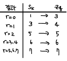
Example) 3-bit image, 64 by 64 pixels

 

 

$s_k$와 $G(z_k)$

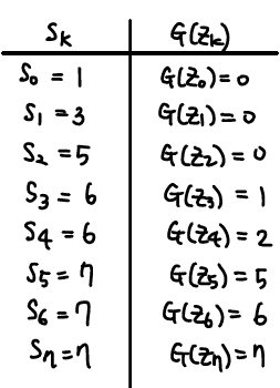
$s_k = \{1,3,5,6,7\}$를 $G(z_k) = \{ 0, 1, 2, 5, 6, 7\}$을 가진다. 제일 비슷한 값끼리 맵핑하게 되면,

 

Comparison between histogram equalization and matching

그림이 여전히 잘 안보이게 된다.

목표한 히스토그램을 얻을 수 있다.

 

Local histogram processing

Global은 entire image기반이다 보니, small area에 대한 효과가 없을 수 있다. 이를 고려하여 pixel 단위로 neighborhod 단위로 histogram을 수행하는 방식이 제안되었다. Histogram statistic 기반의 image enhancement 과정이라고 보면 된다.

 

• $r$ in [0, L-1]
• $p(r_i)$ : normalized histogram value of $r_i$ intensity
• $n^{th}$ moment : $\mu_n(r) = \sum_{i=0}^{L-1} (r_i - m)^n p(r_i)$
• mean : $m = \sum_{i=0}^{L-1} r_i p(r_i)$
• variance: $\sigma^2 = \mu_2(r) = \sum_{i=0}^{L-1} (r_i - m)^2 p(r_i)$

 

가령 local enhancement가 이렇게 가능하다.

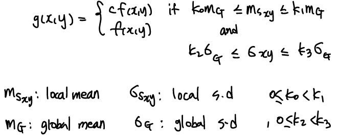
적절한 $c$와 $k_i$를 통해 이미지 퀄리티가 높아질 수도 있다. 대충 local이 global과 다른 패턴일 경우 pixel을 강화하는 느낌이다.

 

Spatial Filtering

Linear Spatial filtering

Linear이므로 연산의 순서는 변할 수 있다. Filtering은 다음처럼 진행된다.

$$g(x,y) = \sum^{a}_{s=-a} \sum^{b}_{t=-b} w(s,t)f(x+s, y+t)$$

 

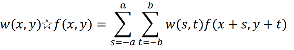
• Spatial correlation

w = [1,2,3,4,5]

• Spatial convolution

w = [5,4,3,2,1]

 

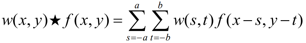
Correlation의 kernel을 180도 돌려서 correlation을 수행하면 convolution 연산이 된다. 또한 kernel이 symmetric하면 180도 돌려도 같으므로 correlation=convolution이 된다. 보통 convolution이 linear spatial filtering으로 사용된다.

 

Padding method

• zero-padding : dark border가 발생할 수 있다.
• mirror-padding : 3 2 | 1 2 3
• replicate-padding : 1 1 | 1 2 3

 

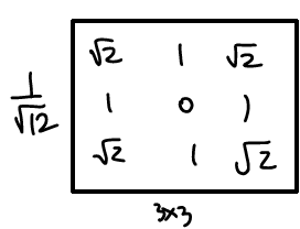
Separable filter kernels

Linear 연산이므로 separable하면 순서를 바꿔서 실행해도 좋다는 장점이 있다. 또한, $M$x$N$ 행렬을 row나 column 하나씩 분해하면 2D 연산을 1D 연산으로 수행할 수 있다.

• Separable : $G(x,y) = G_1(x,y)G_2(x,y)$

 

$$w*f = (w_1*w_2)*f = (w_2*w_1)*f = (w_1*f)*w_2$$

 

Construct spatial filter

1. 수학적인 접근
   1. Averaging : 이미지 블러링
   2. Local derivate : 이미지 sharpening
2. 2D 공간 샘플링 기반
   1. Gaussian fucntion -> weighted-average(lowpass) filter 구현 가능
3. 주파수 응답 기반
   1. Fourier transform 기반의 도메인 변경

 

Smoothing (lowpass) Spatial Filters

Smoothing은 high frequency component를 줄이는 방식으로 sharpeness와 noise를 제거하는 데 사용된다.

 

Box filter

Filter의 크기가 커질수록 블러링 효과가 강해진다.

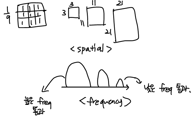
Averaging filter라고 생각하면 된다.

 

Lowpass Gaussian Filter Kernels

3x3 행렬 예시

 

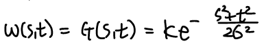
가우시안 커널의 max size는 $6\sigma$의 올림 값이다. 주로 odd size로 사용한다. Max가 정해진 이유는 $6\sigma$면 거의 99% 이상 커버가 되기 때문이다.

 

만약 $\sigma$가 7이면, 43x43 filter를 사용하게 된다. 41도 괜찮지만 43이 더 많은 정보를 포함할 수 있기 때문이다.

 

가우시안 함수의 product와 convolution은 또한 가우시안 함수를 가지는 것도 장점이다.

 

Box filter vs Gaussian filter

• 가우시안 커널이 박스 필터와 동일한 블러링 효과를 얻기 위해서는, 박스 필터보다 커야함
• 가우시안 커널은 $6\sigma$보다 크기가 커져도, 거의 효과 변화가 없음
• 가우시안이 edge에서 조금 더 smooth하게 blur됨
• 보통 blur 필터는 이미지 크기에 영향을 많이 받음
  • 이미지 크기가 커지면, kernel 크기와 standard deviation도 커져야 같은 효과의 blur 가능

 

Order-statistic filters (nonlinear)

Median filter

Neighborhod 중에 중위값을 사용하는 방식이다. Sorting 기반이기 때문에, real-time은 어려우며 주로 blur 효과 없이 노이즈를 제거하는 목적으로 사용된다.

 

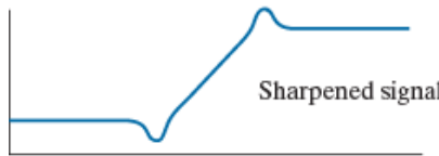
Sharpening (highpass) Spatial Filters

• Intensity 사이 변화를 강조하는 것이 목표이다.
• High frequency components in Fourier domain
• Spatial differentiation이 사용된다.

• First derivative
  • Constant intensity에서는 0임
  • Intensity 변화 시작에서는 0이 아님
  • Intensity 변화 구간에서도 0이 아님
• Second derivative
  • Constant intensity에서는 0임
  • Intensity 변화 시작에서 0이 아님
  • Intensity 변화 구간에서 0임

 

정리하면, first derivative는 밝기 변화의 크기를 측정하지만 변화가 유지되는 구간에서는 두꺼운 edge를 생성한다. 이는 edge를 넓게 나타나게 만든다.

 

Second derivative는 1 pixel 정도의 두께로 경계선을 구분하며 더 얇은 edge를 검출할 수 있다. 그러므로, second derivate는 first보다 sharpening에 적합하다.

 

대표적인 second derivative는 Laplacian이다.

 

Laplacian

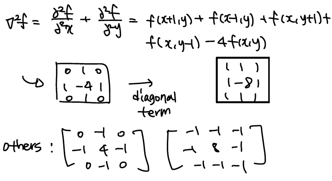
Sharpening : $g(x,y) = f(x,y) + c \left[ \nabla^2 f(x, y) \right]$

 

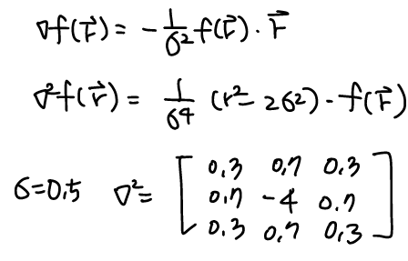
Gradient and Laplacian operation using Gaussian function

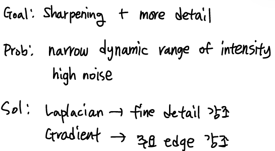
가우시안 블러링을 통해 이미지의 노이즈를 줄이고, gradient와 laplacian 연산을 통해 edge 감지와 sharpening을 수행할 수 있다. Gradient는 first derivative로 edge를 찾는 데 유용하고 laplacian은 second derivate로 edge를 강조할 수 있다.

 

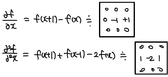
• Approximate gradient : $\nabla I = \nabla f * I$
• Approximate laplacian : $\nabla^2 I = \nabla^2 f * I$

 

실제로 미분하면 다음과 같다.

 

Unsharp masking and highboost filtering

High-frequency part를 강조하여 이미지 디테일을 살리는 방법이다.

(1) smoothing image, $f_{smooth}(x,y)$

(2) unsharp mask = $f-f_{smooth}$

(3) $g(x,y) = f(x,y) + k*\left[ f-f_{smooth} \right]$  ($k>1$)

 

강조된 intensity가 negative를 가질 수 있으므로, 전체적인 intensity 증가 필요성이 있다. 그리고 $k$가 커지면 edge가 두꺼워지기도 한다.

 

First-order derivate로 이미지 sharpening (gradient)

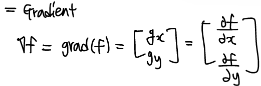
Gradient의 크기는 벡터의 길이로 표현된다.

$$M(x,y) = || \nabla f || = \sqrt(g_x^2 + g_y^2)$$

$$M(x,y) \approx |g_x| + |g_y|$$

Gradient Image; edge 검출에 좋다

 

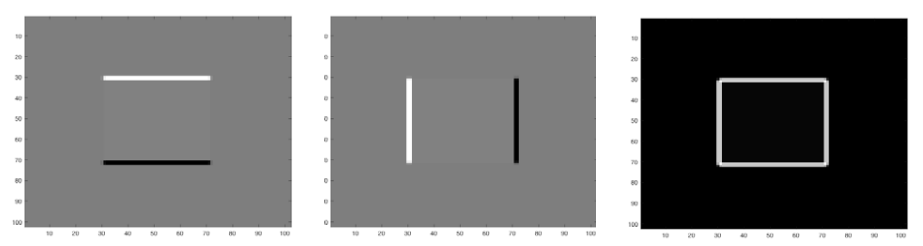
이 외에도 gradient 기반의 검출 방법이 있다.

 

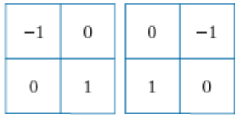
Robert Cross-gradient Operators, $M(x,y) \approx |z_9-z_5| + |z_8-z_6|$

Sobel Operators

vertical edge / horizontal edge

 

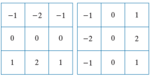
Gradient는 edge enhancement에 사용되며, edge에서의 작은 변화도 잘 보여주는 장점이 있다.

 

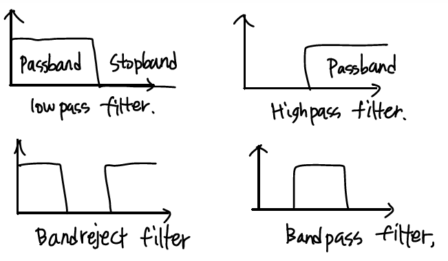
Highpass, Bandreject, Bandpass filters

 

Combine all!

(1) Laplacian으로 edge 검출

(2) I + (1) = edge 강조

(3) Sobel(I) = edge 주변 value 감소

(4) Box filter on (3)

(5) (4)*(1) = mask (edge 주요)

(6) I + (5)

(7) 어두우니까 power-law transformation