2. ML overview, Visual Features for ML, Language Model & Word Embedding, Neural Network, Convolutional Neural Network, Recurrent Neural Network
기말고사를 대비하기 위한 글이다.
ML overview
1. Types of learning
| Supervised | Unsupervised (self-supervised) |
|
| Discrete | Classification | Clustering |
| Continuous | Regression | Dimensionality Reduction |
2. Classification
대표적인 모델은 K-NN, Logistic regression, SVM이 있다.
| K-NN | f(x) = laber of the nearest training data |
| Logistic regression | 모델 결과값에 따라 분류한다. |
| SVM | 2개 class 분류를 잘하는 hyper-plane을 찾는 모델이다. * hyper-plane : wTx+b * classifiaction : f(wTx+b) margin을 maximize하는 weight를 찾으면 된다. * p=2wT |
3. Classification issue
- Multi-class classification
- Non-linear separable
Visual Feature for ML
1. Bag of Features
다음의 과정을 거쳐서 visual vocabulary를 뽑는 것이 목표이다.
- Feature extraction (patch로 뽑음 ex) SIFT)
- Learning the visual vocabulary (Clustering+Center feature)
- Quantize the visual vocabulary
- Represent images by frequencies of visual words
- Train the model (ex) SVM)
2. Visual word 이용의 Pros and Cons
| Pros | Cons |
| Flexible to geometry, deformation, viewpoint Image content 요약 good Fixed sized dimensional vector Good in practice |
Background 정보, Foreground 정보 mixed인 경우 - Instance를 잘 표현했는가? - Optimal인가? 의 문제가 제기됨 |
3. Spatial Pyramid Representation
위의 방식은 Spatial 정보와 Layout 정보가 잘 표현되는지 문제가 제기될 수 있다. 이에 다른 해상도로 여러 vocabulary를 뽑는 방법을 제안한다.

Language Model & Word Embedding
1. Word Vectors
Context에 따라서 word를 set of word로 표현한다. Frequently appear하는 word로 목표 word의 의미를 결정하는 방식이다.
2. Word2Vec
위의 방식처럼 count하지 않는다. Word embedding의 일환으로서 weight를 사용해 word를 vector로 표현한다. 2가지 방식이 있다.
Skip-Gram Task
다음의 과정을 통해서 context word를 vector화 한다.
- Target word와 context word를 (+)로 설정한다.
- Randomly sample을 통해서 (-) word를 선택한다.
- Logistic Regression을 이용해서 두 케이스에 대한 classification model을 생성한다.
- 이 때의 weight를 이용해서 word embedding한다.
CBOW Task
Skip-gram 방식과 다르게 context를 이용해서 target word를 벡터화 한다.
3. Word vector 사이에 Relation을 가지는 결과를 얻게 된다.
ex) vector('king') - vector('man') + vector('woman') = vector('queen')
Neural Network
1. Deep Learning
DL에서는 feature도 model이 알아서 찾는 것이 목표이다.
모델은 f(x)와 G.T의 값을 비교하여 Loss가 최소화 되도록 weight를 업데이트하는 것이 목표이다.
구성은 Data, Model, Loss function, Optimizer로 이루어진다.
Neural Network : Optimization
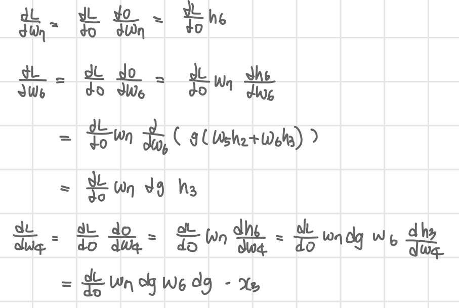
1. Backpropagation
근본적인 규칙은 chain-rule을 이용한다는 것이다.
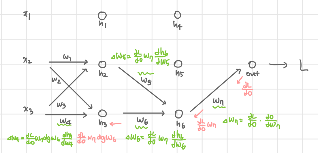
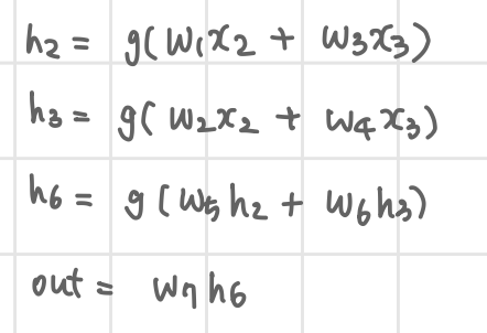
위와 같은 4 layer(Input-Hidden-Hidden-Output)를 가지는 네트워크가 있다고 가정하자.
x3의 Forward 결과는 아래와 같다.
Loss는 간단하게 설정하여 다음과 같다.
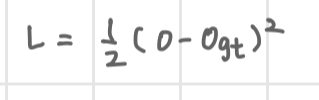
Forward 정보와 Loss를 이용해서 Backpropagation을 수행한다.
핵심은 dLdwn를 구한다는 것을 기억하는 것이다.
Backpropagation의 과정은 다음과 같다.
2. Optimizer
Weight를 업데이트 하는 방식을 효율적으로 하기 위한 노력이다. 현재는 다음과 같이 굴직한 방법들이 제안되었고 Adam을 주로 사용한다.
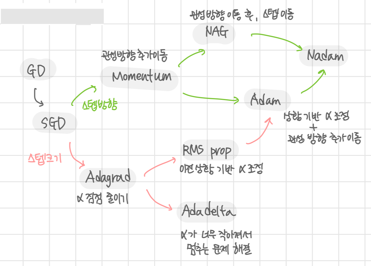
*GD, SGD, Adagrad, RMS prop, Momentum, Adam이 중요
Neural Network : Activation, Regularization
Activation은 model에 non-linearity를 주기 위해 필요하다. Model이 linear하다면, 그냥 함수를 사용하는 것과 다르지 않기 때문이다.
1. Sigmoid
f(x)=11+e−x
Saturation과 Kill gradient 문제가 있다. 값이 0~1로 결정되기 때문에 gradient flow가 흐르지 않을 수 있다. 또한 weight가 너무 크면 saturate될 가능성이 있다.
*Derivate: f′(x)=f(x)(1−f(x))
2. Tanh
f(x)=21+e−2x−1
Saturation될 수 있다. Output이 zero-centered이다.
*Derivate: f′(x)=1−f(x)2
3. ReLU
f(x) = 0 if x < 0 else x
간단한 식으로 train이 빠르다는 장점이 있다. Linear이기 때문에 saturation되지 않는다. 표현력이 좋고 vanishing gradient problem이 없다. 다만 Dead ReLU 케이스가 존재한다. 이에 대해서는 soft ReLU 등의 대안이 존재한다.
4. Dropout
f(x) = x if px > p else 0
Forward 과정에서 randomly 뉴런을 죽이는 방식이다. 일반적으로 p=0.5이다. Netowork가 중복되는 표현을 가지지 않도록 만들어 준다.
5. Batch Normalization
학습이 faster, stable해진다. Batch에 대해서 re-centering, re-scaling을 수행하여 mean=0, unit variance를 가지도록 만드는 것이 목표이다. 또한 learnable learning rate를 사용한다.
γ=√var(x), β=E[x]
CNN
1. Convolution Layer
Convolution layer의 결과는 다음과 같은 크기를 가지게 된다.
- w : width
- h : height
- f : filter size
- p : padding size
- s : stride size
wout=win−f+2ps+1
hout=hin−f+2ps+1
cout = number of filters
2. Pool Layer
Pooling layer의 결과는 다음과 같은 크기를 가지게 된다.
wout=win−fs+1
hout=hin−fs+1
Dout=Din
3. Fully Connected Layer
일반적으로 1차원 벡터를 입력으로 받는다.
Input : (1, 555)
w : (10, 555)
Output : (1, 10)
4. Conv layer의 Parameters, Memory, FLOPS
| # of parameters | memory | FLOPS |
| f∗f∗cin∗cout | (c∗w∗h)out∗32/8 | f∗f∗cin∗(c∗h∗w)out |
5. Pool layer의 Parameters, Memory, FLOPS
| # of parameters | memory | FLOPS |
| none | (c∗w∗h)out∗32/8 | f∗f∗(c∗h∗w)out |
6. FC layer의 Parameters, Memory, FLOPS
| # of parameters | memory | FLOPS |
| cin∗cout | cout∗32/8 | cin∗cout |
CNN Application : Computer Vision
1. R-CNN
Region proposal된 영역에 대해서 CNN 수행
얻은 Feature로 SVM 수행
2. Fast R-CNN
전체 영역에 대해서 CNN 수행, Region proposal로 영역 얻음
Pooling하고 FC 수행해서 feature 얻음
얻은 feature에 대해서 Linear layer+softmax를 통해 classification하거나 Linear만으로 Bounding Box regressor 역할을 수행할 수 있음.
3. Faster R-CNN
Fast R-CNN을 2번 수행한다고 보면 된다.
Fast R-CNN을 통해서 Bounding Box를 얻어낸다.
전체 이미지에 Conv을 했던 feature map에서 해당 영역에 대해 classification하거나 다시 Box regressor을 한다.
4. YOLO
Image를 Conv를 통해서 7×7×(?) feature map을 얻어낸다.
2개의 FC layer를 통해서 예측값을 얻어낸다.
예측값은 " B×5 + # of class "이다.
- B : Box 내 예측할 object 수
- 5 : (x,y,w,h, confidence)
- # of class : 전체 class 수
논문에서의 결과는 B=2, class=20의 결과이다.
따라서 예측값은 30의 dimension을 가지게 된다.
따라서 최종 feature map 크기는 7×7×30 이다.
Recurrent Neural Network
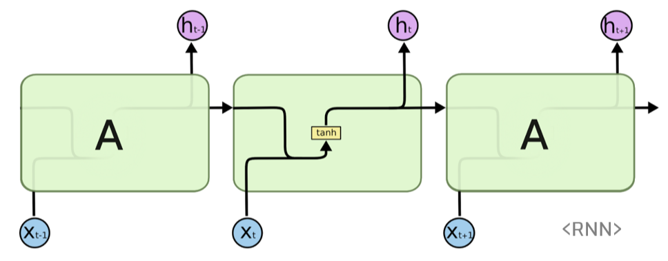
1. Vanilla RNN
심플한 모델이다. Input에 대해서 Forward를 수행하고 outputt와 ht를 결과값으로 내보낸다. NLP에 주로 사용되며 간단한 구조로 인해 긴 문장에 대해서 초반 단어들의 영향력이 사라진다는 단점을 가지고 있다. 이를 해결한 것이 LSTM이다.
Model
Fowrading
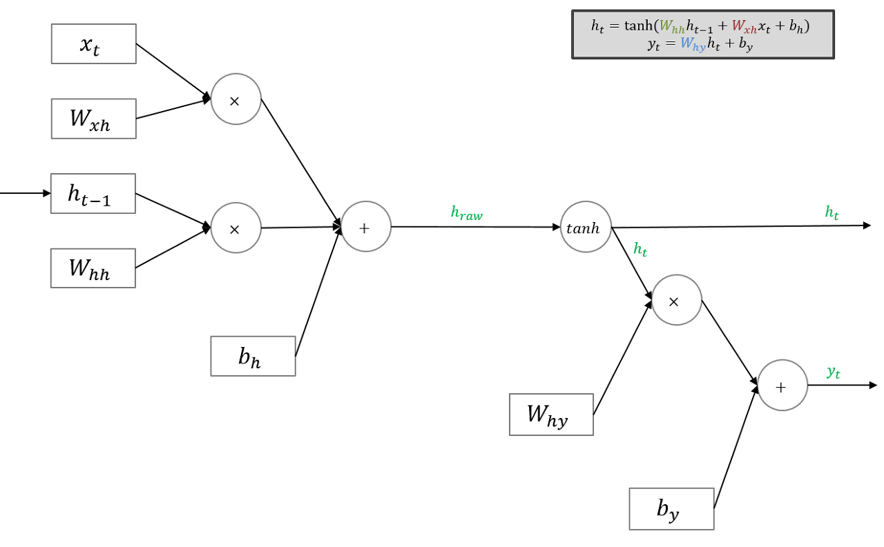
위 블로그에 더 자세한 설명이 되어 있다.
초기 입력에 대한 ht−1은 zero vector로 설정하면 된다.
Many to one RNN의 경우 마지막 Input에 대해서만 yt를 구하면 된다.
Forwarding은 위 과정처럼 진행된다.
Backwarding
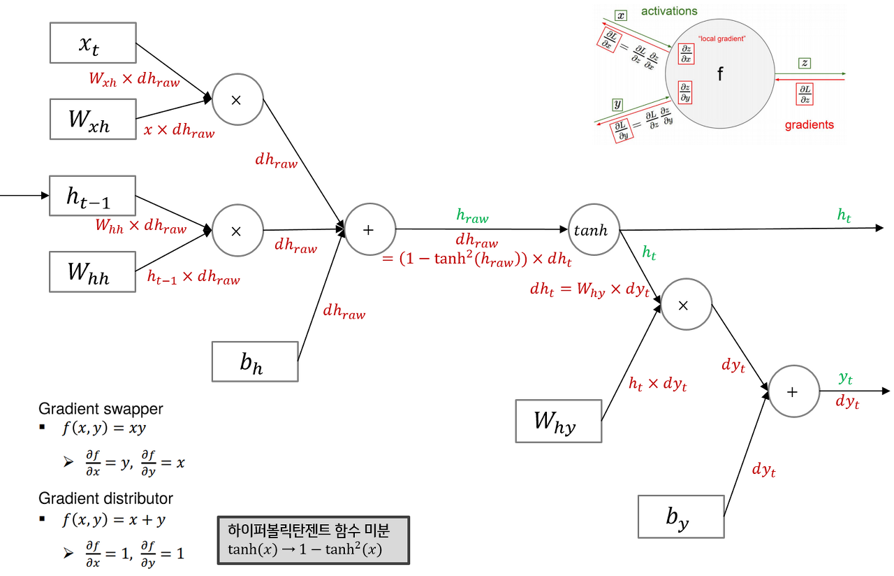
Many to one의 backward는 dht=Why∗dyt+dht+1이라고 생각하면 된다.
위 그림의 구조에서 gradient flow는 +의 경우 그대로 흐르며, ×인 경우 반대의 variable을 곱해서 gradient로 사용하면 된다.
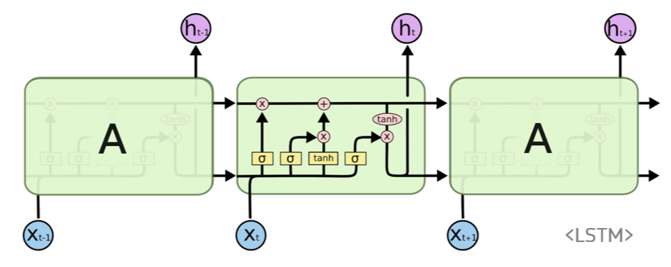
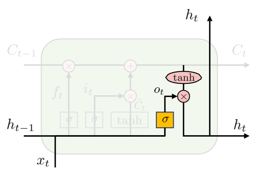
2. LSTM
RNN의 단점을 보완하기 위해 previous state 정보인 cell state를 추가하며 여러 gate를 사용해 정보의 손실률을 결정한다.
Gate에서는 linear interaction만 수행하기 때문에 vanishing gradient 문제를 해결할 수 있다.
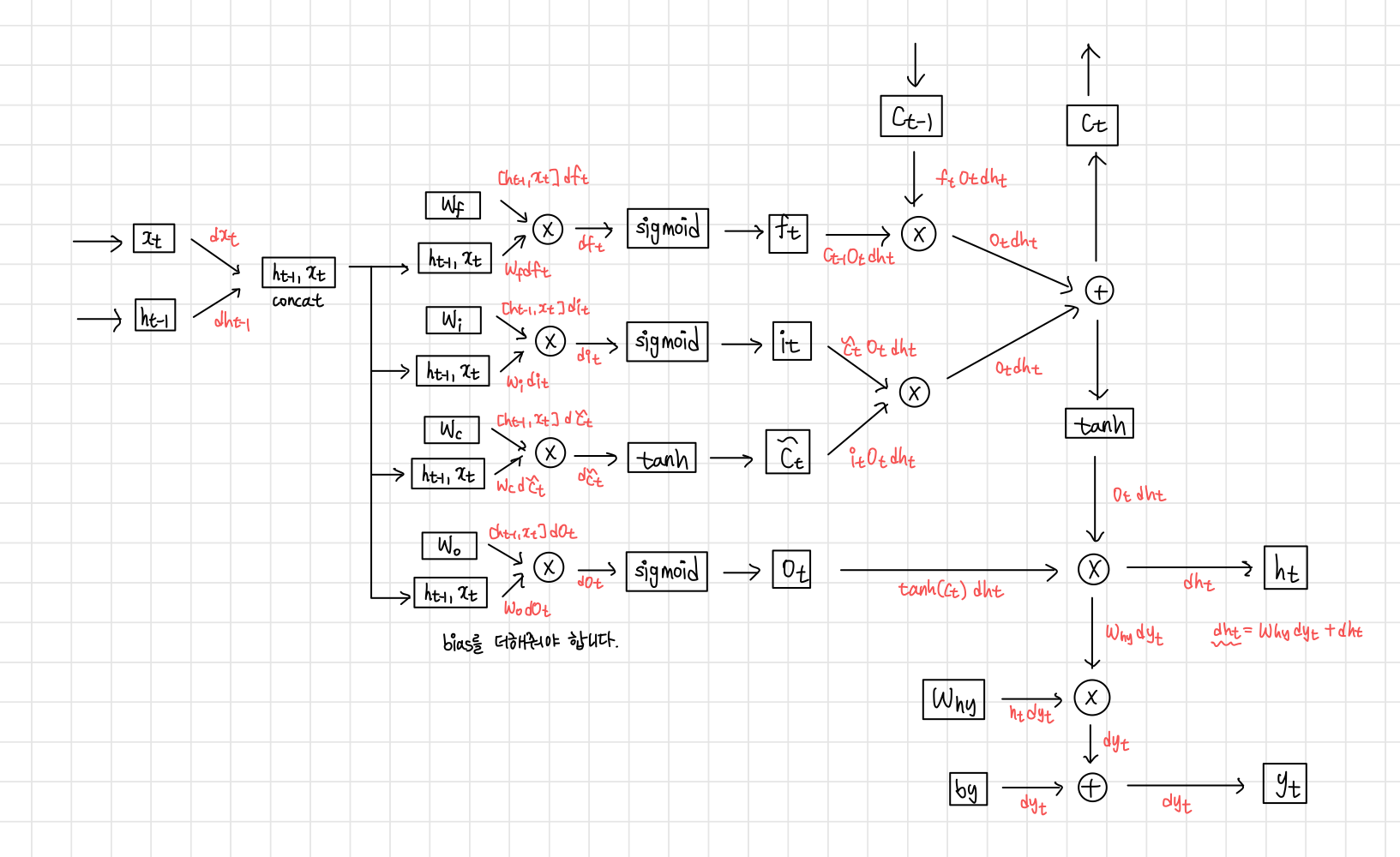
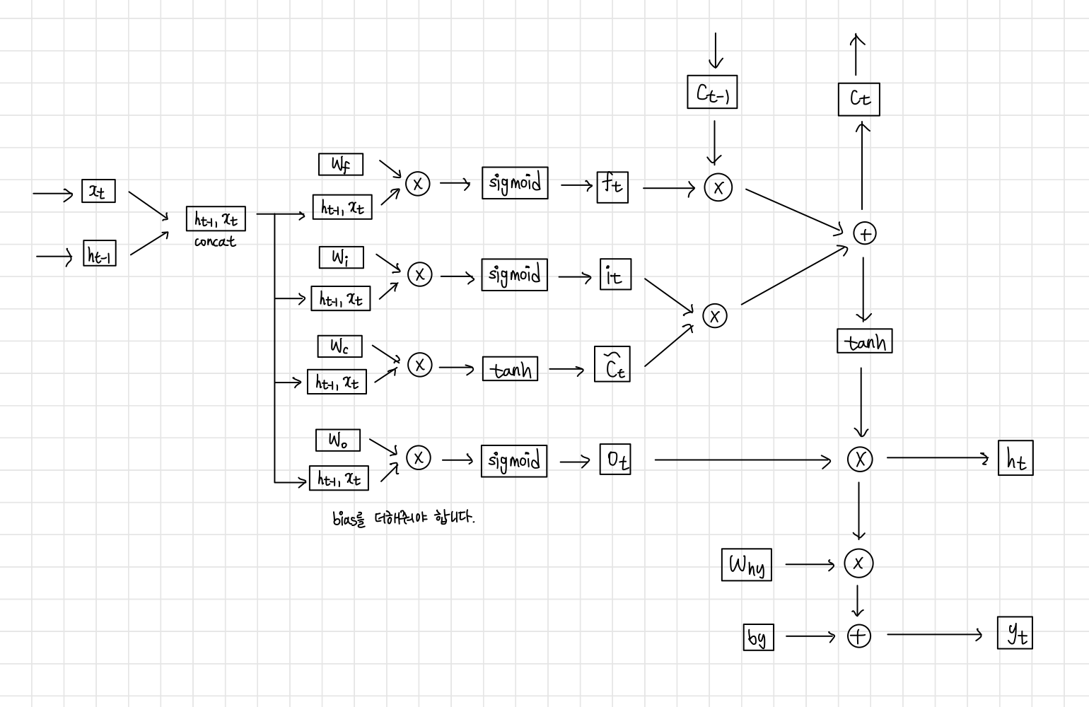
Model
Forwarding
다음의 flow를 따른다.
- Forget Gate
ht−1 과 xt를 보고 cell state를 얼마나 잊을 건지 0~1로 결정
Sigmoid function을 사용한다.
ft=sigmoid(Wf[ht−1,xt]+bf)

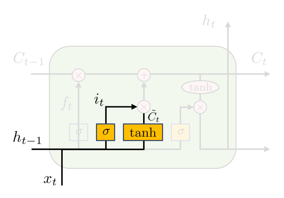
- Input gate
어느 정보가 cell state에 저장될 것인지 결정한다.
새로운 cell state 정보가 tanh으로 생성된다.
it=sigmoid(Wi[ht−1,xt]+bi)
ct,new=tanh(Wc[ht−1,xt]+bc)
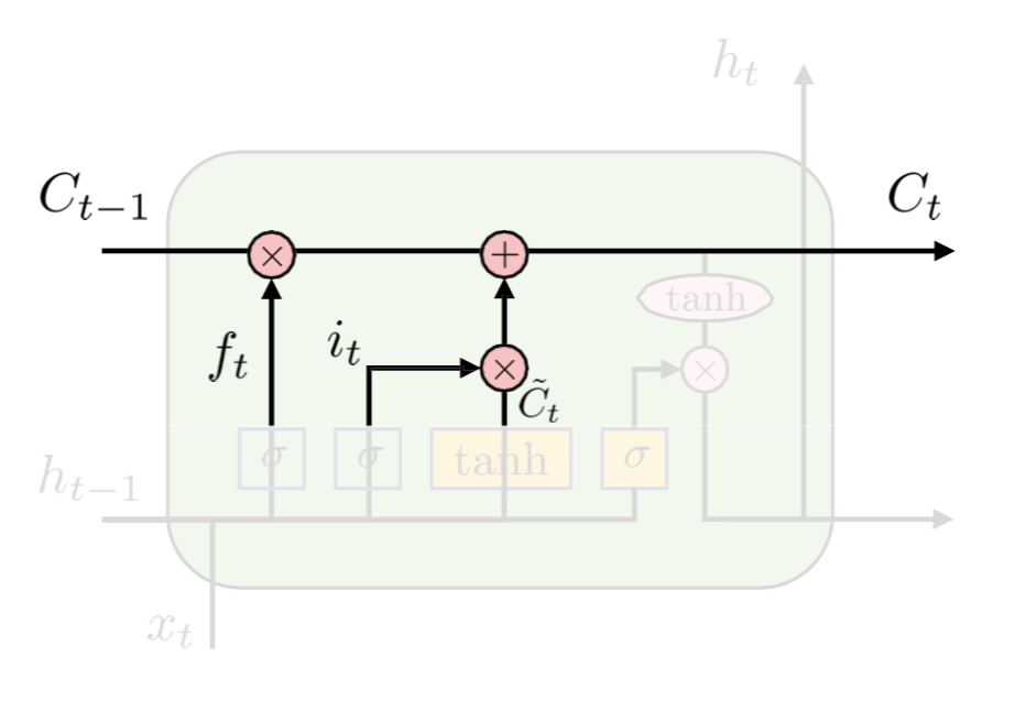
- Update old cell state
Cell state를 업데이트한다.
ct=ft∗ct−1+it∗ct,new
- Output gate
Cell state 중 어느 part가 output이 될지 결정한다.
이를 위해 ct를 tanh으로 activation map을 얻는다.
ot=sigmoid(Wo[ht−1,xt]+bo)
ht=ot∗tanh(ct)
- 전체 과정
Backpropagation
RNN에서 구했던 것처럼 수행하면 된다.